NFL Predictions Using Machine Learning
Goal
The purpose of this project is to practice applying Machine Learning on NFL data. After taking Andrew Ng’s Machine Learning course, I wanted to re-write some of the methods in Python and see how effective they are at predicting NFL statistics. Using Las Vegas as a benchmark, I predicted game winners and the spread in these games.
Overview
-
The first step was acquiring the data. For this, I webscraped the statistics from Pro Football Reference using Beautiful Soup. My Python code for this is on Github. The code collects data from boxscores and creates .json files, where there is a file for each year and team, and the contents is a dictionary containing the webscraped statistics for each game week.
-
These .json files were then used to create .csv files for analysis in Python using Pandas and Numpy. For first models, I used logistic regression for predicting game winners, and linear regression for predicting the spread.
-
For my training set, I chose data from years 2009, 2011, and 2013. For my cross-validation set, I used years 2010 and 2012. Year 2014 was used as my test set.
-
Results up until now are located at the bottom of the page.
What is the Vegas line?
Let’s start with an example (my favorite example). In Super Bowl XXXII on January 25, 1998, the Vegas Line for the game between the Green Bay Packers and Denver Broncos was ‘Green Bay Packers -11.0’. This means that the Green Bay Packers were favored to win the game by 11 points. If you bet on Green Bay, then they had to beat the Denver Broncos by more than eleven points for you to win the bet. Alternatively, if you bet on the underdog Broncos, you would win if they won the game or lost by up to 11 points. The Broncos won the game by 7 points, thanks in part by John Elway’s infamous helicopter dive, so the actual line for the game was ‘Denver Broncos -7.0’, and so Las Vegas’s prediction was 18 points off.
In my model, I changed the line definition slightly for ease of use. I specified the line always in terms of the home team, so a negative value means that the home team is favored, and a positive value means they are the underdog. Thus, when I predict the line, I just predict a single value for the home team that can take on positive and negative values.
How Good is Vegas?
The following histogram shows how successful Las Vegas Lines have been from 2011-2014. As the figure shows, the data closely resembles a normal distribution. Negative x-values correspond to the Vegas favorite losing the spread, but not necessarily the game.

The figure below compares the Vegas Line for home teams to how the home team actually performs. For example, the point at (-10, -58) corresponds to the December 9, 2012 game between the Arizona Cardinals and the Seattle Seahawks. The Vegas Line was -10 for Seattle, but they actually won 58-0. Vegas correctly predicting the game would correspond to a dot along the dashed line labeled as the ‘Line of Perfect Prediction.’ The color values indicate density, and demonstrate that Vegas is very good at predicting close games.

One might assume that Las Vegas predictions are much worse at the beginning of the season and then improve as time goes on and more data is acquired. However, the figure below seems to contradict this intuition. There is very little correlation between the two, except for the low variance at the end of the season.

Another idea I wanted to test was how good Vegas is as a function of their line. In other words, are they better at predicting blowouts or predicting close games? The figure below plots the mean and standard deviation of the absolution distance of the Vegas Line to the actual line (minimum 10 data points per Vegas Line). There isn’t much correlation here, but they are slightly better at predicting close home losses. The high standard deviation is further proof that it is very hard to predict NFL scores.

The following figure shows the frequency of final score distributions and how Vegas compares to it. As the figure shows, the most commonly occuring are +/- 3 and +/- 7, and Vegas mimics this. This makes sense because many games are decided by a single field goal or touchdown. In my opinion, this figure is very interesting because not only does Vegas try to predict the line, they also try to match the score frequency.

The table below shows how successful Vegas is at predicting game winners. This is the benchmark that I compared my code to.
| Year | % Correct |
| 2009 | 69.53 |
| 2010 | 65.74 |
| 2011 | 66.41 |
| 2012 | 64.17 |
| 2013 | 68.50 |
| 2014 | 67.73 |
| Overall | 67.02 |
Predicting Game Winners
Since predicting the winner of an NFL game is a classification problem, logistic regression is a good starting model.
Logistic Regression Model Description
For this model, I calculated the average year-to-date value for each variable. Since averages early in the season will be less accurate, all row data is taken from weeks 5 to 17. In order to determine which variables to use, I experimented with different options, choosing those that performed best in the training set. Then I chose my final model based on which performed best in the cross-validation set.
The variables that I chose are:
-
Home and Away winning percentages (2)
-
Home team’s home winning percentage (1)
-
Away team’s away winning percentage (1)
-
Points Scored and Points allowed for both teams (4)
-
3rd Down Efficiency on Offense and Defense for both teams (4)
-
Touchdown Scoring Efficiency (Touchdowns / Drives) on Offense and Defense for both teams (4)
-
Defensive Turnovers for both teams (2)
-
Quarter 1 scoring for both teams (2)
Thus I used 20 variables (21 if you count x_0)
Logistic Regression Results
Below are the weights for each of the normalized parameters, listed from most important to least important.
| No. | Variable | Value |
| 1 | Away Off. Touchdown Efficiency | -9.41 |
| 2 | Home Off. Touchdown Efficiency | 5.41 |
| 3 | Away Off. 3rd Down Efficiency | 4.41 |
| 4 | Home Def. Touchdown Efficiency | -4.38 |
| 5 | Away Def. Touchdown Efficiency | -3.94 |
| 6 | Away Def. 3rd Down Efficiency | 1.27 |
| 7 | Home Def. 3rd Down Efficiency | 1.09 |
| 8 | Home at Home Winning Percentage | -0.79 |
| 9 | Away Winning Percentage | -0.60 |
| 10 | Home Winning Percentage | -0.46 |
| 11 | Home Off. 3rd Down Efficiency | -0.37 |
| 12 | Away Def. Turnovers | 0.18 |
| 13 | Home Def. Turnovers | -0.14 |
| 14 | Away Road Winning Percentage | -0.11 |
| 15 | Home Points Allowed | -0.096 |
| 16 | Home Points Scored | 0.083 |
| 17 | Away Points Allowed | 0.054 |
| 18 | Away Quarter 1 Scoring | -0.020 |
| 19 | Away Points Scored | 0.015 |
| 20 | Home Quarter 1 Scoring | 0.0075 |
| 21 | y-intercept | 0.0017 |
The table below shows the success of my logistic regression model across all three data sets, as well as Vegas’s success on the same data sets.
| % Correct | Vegas % Correct | |
| Training Set | 66.84 | 67.76 |
| Cross-Validation Set | 66.150 | 67.73 |
| Test Set | 66.154 | 69.47 |
As listed above, Vegas correctly predicted 69.47 percent of games in my test set (weeks 5-17 of the 2014 season). Getting within a few percent of Las Vegas’s predictions using a straightforward logistic regression model was much better than I anticipated!
The following table shows that my logistic regression model and Las Vegas agree over 88% of the time. This is based on results from the test set.
| % Vegas Correct | % Vegas Incorrect | |
| % Log. Reg. Correct | 62.96% | 4.76% |
| % Log. Reg. Incorrect | 6.88% | 25.40% |
Why does this model work so well?
At first, it was surprising to me that statistics such as passing yards, rushing yards, sacks, etc. didn’t have as big of an effect on the outcome of a game as the variables listed above. But I think it makes sense. 3rd down efficiency tells you how good a team is at moving the ball down the field. Touchdown scoring efficiency tells you how good a team is at finishing drives. Teams that regularly put points on the board in the first quarter can stick to their gameplan and not spend the game digging themselves out of a hole. A lot of the other statistics are included in these numbers. Offenses that turnover the ball over frequently or get sacked a lot are not going to be as effective at converting on 3rd down and scoring. And garbage time stats drown out the effectiveness of passing and rushing yards.
Predicting the Spread
Predicting the spread is a regression problem, so the first model to try is linear regression. The value that we want to minimize is the absolute distance of the predicted line to the actual value.
Linear Regression Model Description
I used the same setup in this problem as the last once, where each variable is the average year-to-date value and all row data is taken from weeks 5 to 17. Variables were chosen based upon what performed best in the cross-validation set.
The variables that I chose are:
-
Home and Away winning percentages (2)
-
Home team’s home winning percentage (1)
-
Away team’s away winning percentage (1)
-
Points Scored and Points allowed for both teams (4)
-
3rd Down Efficiency on Offense and Defense for both teams (4)
-
Touchdown Scoring Efficiency (Touchdowns / Drives) on Offense and Defense for both teams (4)
-
Defensive Turnovers for both teams (2)
-
Quarter 1 scoring for both teams (2)
-
Quarter 2 scoring for both teams (2)
So there are 23 variables including x_0.
Linear Regression Results
Below are the weights for each of the normalized parameters, listed from most important to least important.
| No. | Variable | Value |
| 1 | Away Off. Touchdown Efficiency | 75.53 |
| 2 | Home Off. Touchdown Efficiency | -34.38 |
| 3 | Away Off. 3rd Down Efficiency | -30.56 |
| 4 | Home Def. Touchdown Efficiency | 16.33 |
| 5 | Away Def. Touchdown Efficiency | -12.54 |
| 6 | Away Def. 3rd Down Efficiency | -7.66 |
| 7 | y-intercept | 6.72 |
| 8 | Away Winning Percentage | 5.48 |
| 9 | Home Def. Turnovers | 2.17 |
| 10 | Home at Home Winning Percentage | 2.10 |
| 11 | Away Def. Turnovers | -1.12 |
| 12 | Home Winning Percentage | 0.76 |
| 13 | Home Off. 3rd Down Efficiency | 0.76 |
| 14 | Home Points Allowed | 0.58 |
| 15 | Home Points Scored | -0.45 |
| 16 | Home Def. 3rd Down Efficiency | -0.35 |
| 17 | Home Quarter 1 Scoring | -0.25 |
| 18 | Away Quarter 2 Scoring | -0.22 |
| 19 | Home Quarter 2 Scoring | -0.21 |
| 20 | Away Points Allowed | -0.20 |
| 21 | Away Points Scored | -0.16 |
| 22 | Away Road Winning Percentage | -0.07 |
| 23 | Away Quarter 1 Scoring | -0.04 |
Below is the table that shows how both my linear regression model and Las Vegas scored in the three data sets. The value measured is the average absolute distance between the predicted line and the actual line. I rounded the linear regression results to the nearest half point to match how Vegas Lines are presented.
| Linear Regression Line | Las Vegas Line | |
| Training Set | 10.92 | 10.82 |
| Cross-Validation Set | 11.07 | 10.86 |
| Test Set | 11.55 | 11.00 |
It is interesting to note that if you look at this table and the logistic regression table above, Las Vegas is most successful at predicting the game winners in the test set (2014) versus the cross-validation and test sets, but that is where they did the worst when predicting the lines. The figure below compares how both Las Vegas and the linear regression model do at predicting the spread. One interesting spot is the accuracy of the linear regression model at x = 3. Along that vertical line, it performs much better than Vegas. Two other interesting points are at x=-8 and x=-6.5. The former has no Vegas predictions, but the latter has many more than its neighbors.

The figure below shows how similar the linear regression model is to the Las Vegas line. As the figure shows, they match pretty well, and there is a definitive trend along the red dashed y=x line. Points in the second and fourth quadrants indicate that there was disagreement on which team was predicted to win, but on the whole, there is not any obvious anomalous data points.
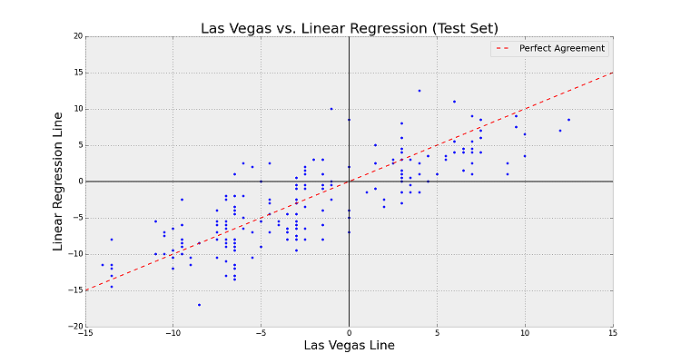
The vertical dots are one interesting artifact in the above figure. These are present because Las Vegas adjusts their lines to follow the frequency of score differentials, as plotted above (see the figure entitled “Frequency of Spreads (2011-2014)”). As the figure below shows, the linear regression model does not follow this frequency. The next question then is will the linear regression model perform better if the predictions are adjusted to match this figure?

Possible Improvements
-
I can increase the accuracy of Touchdown Scoring Efficiency by parsing the data more carefully. For instance, a team that kneels down to end the game shouldn’t have that drive included. Another idea might be to have a way of dealing with garbage time points.
-
Getting more data. This might not be entirely beneficial, since league changes have led to increased scoring and passing yards.
-
Accounting for injuries. Injuries to key players can definitely alter the outcome of the game.
2015 Success
Summary of Results
The table below is a summary of how my models have performed against Vegas so far this year. Since my models only use data from weeks 5-17, I start the table at Week 5. ‘Vegas Line Dist’ and ‘Lin. Reg. Line Dist’ are measures of the average absolute distance of all the predicted lines to the actual lines for all games that week. ‘Lin. Reg. Beat Vegas’ is the number of times the linear regression predicted line is closer to the actual line than Vegas’s prediction.
| Week | Vegas Picks | Log. Reg. Picks | Vegas Line Dist | Lin. Reg. Line Dist | Lin. Reg. Beat Vegas |
| 5 | 10/14 = 71.43% | 11/14 = 78.57% | 7.46 | 9.00 | 5/14 = 37.71% |
| 6 | 8/14 = 57.14% | 10/14 = 71.43% | 9.36 | 9.07 | 8/14 = 57.14% |
| 7 | 11/14 = 78.57% | 9/14 = 64.29% | 6.82 | 8.93 | 5/14 = 37.71% |
| 8 | 10/14 = 71.43% | 9/14 = 64.29% | 10.71 | 10.96 | 8/14 = 57.14% |
| 9 | 8/13 = 61.54% | 8/13 = 61.54% | 7.46 | 6.92 | 6/13 = 46.15% |
| YTD | 47/69 = 68.12% | 47/69 = 68.12% | 8.38 | 9.01 | 32/69 = 46.38% |
Weekly Results
Below are the results of how both my models and Vegas’s lines perform from week 5 until now. The Logistic Regression H-value is the predicted output from 0 to 1, where 1 represents a predicted home team victory and 0 a home loss. The closer the value is to 0.5, the more evenly the teams are matched. Bold values for the predicted lines indicated which one is closer to the actual line, and bold values for the picks indicate correct picks.
Week 5 Results
| No. | Home | Away | Home Pts | Away Pts | Actual Line | Vegas Line | Lin. Reg. Line | Vegas Pick | Log. Reg. Pick | Log. Reg. H-val |
| 1 | ATL | WAS | 25 | 19 | -6 | -7.0 | -11.0 | ATL | ATL | 0.743 |
| 2 | BAL | CLE | 30 | 33 | 3 | -6.0 | -5.5 | BAL | BAL | 0.686 |
| 3 | CIN | SEA | 27 | 24 | -3 | -3.0 | -14.5 | CIN | CIN | 0.903 |
| 4 | DAL | NWE | 6 | 30 | 24 | 9.0 | 1.5 | NWE | NWE | 0.287 |
| 5 | DET | ARI | 17 | 42 | 25 | 3.0 | 11.5 | ARI | ARI | 0.211 |
| 6 | GNB | STL | 24 | 10 | -14 | -9.0 | -11.0 | GNB | GNB | 0.846 |
| 7 | HOU | IND | 20 | 27 | 7 | -2.0 | -0.5 | HOU | IND | 0.477 |
| 8 | KAN | CHI | 17 | 18 | 1 | -9.0 | -10.5 | KAN | KAN | 0.648 |
| 9 | NYG | SFO | 30 | 27 | -3 | -6.5 | -10.5 | NYG | NYG | 0.786 |
| 10 | OAK | DEN | 10 | 16 | 6 | 4.0 | 0.5 | DEN | DEN | 0.498 |
| 11 | PHI | NOR | 39 | 17 | -22 | -6.0 | -4.5 | PHI | PHI | 0.746 |
| 12 | SDG | PIT | 20 | 24 | 4 | -3.5 | 3.0 | SDG | PIT | 0.277 |
| 13 | TAM | JAX | 38 | 31 | -7 | -2.5 | -2.0 | TAM | TAM | 0.577 |
| 14 | TEN | BUF | 13 | 14 | 1 | 1.0 | -5.5 | BUF | TEN | 0.658 |
Week 6 Results
| No. | Home | Away | Home Pts | Away Pts | Actual Line | Vegas Line | Lin. Reg. Line | Vegas Pick | Log. Reg. Pick | Log. Reg. H-val |
| 1 | BUF | CIN | 21 | 34 | 13 | 3.0 | 4.0 | CIN | CIN | 0.450 |
| 2 | CLE | DEN | 23 | 26 | 3 | 3.5 | 0.0 | DEN | DEN | 0.468 |
| 3 | DET | CHI | 37 | 34 | -3 | -3.0 | -2.0 | DET | DET | 0.502 |
| 4 | GNB | SDG | 27 | 20 | -7 | -10.5 | -9.0 | GNB | GNB | 0.757 |
| 5 | IND | NWE | 27 | 34 | 7 | 9.5 | 6.5 | NWE | NWE | 0.226 |
| 6 | JAX | HOU | 20 | 31 | 11 | -2.5 | 0.5 | JAX | HOU | 0.428 |
| 7 | MIN | KAN | 16 | 10 | -6 | -3.5 | -5.0 | MIN | MIN | 0.501 |
| 8 | NOR | ATL | 31 | 21 | -10 | 3.0 | 5.0 | ATL | ATL | 0.212 |
| 9 | NYJ | WAS | 34 | 20 | -14 | -7.0 | -8.5 | NYJ | NYJ | 0.824 |
| 10 | PHI | NYG | 27 | 7 | -20 | -5.0 | -3.5 | PHI | PHI | 0.691 |
| 11 | PIT | ARI | 25 | 13 | -12 | 3.5 | 2.5 | ARI | ARI | 0.383 |
| 12 | SFO | BAL | 25 | 20 | -5 | 2.0 | 4.5 | BAL | BAL | 0.284 |
| 13 | SEA | CAR | 23 | 27 | 4 | -7.0 | 0.5 | SEA | CAR | 0.468 |
| 14 | TEN | MIA | 10 | 38 | 28 | -2.0 | -7.5 | TEN | TEN | 0.772 |
Week 7 Results
| No. | Home | Away | Home Pts | Away Pts | Actual Line | Vegas Line | Lin. Reg. Line | Vegas Pick | Log. Reg. Pick | Log. Reg. H-val |
| 1 | ARI | BAL | 26 | 18 | -8 | -8.0 | -15.5 | ARI | ARI | 0.909 |
| 2 | CAR | PHI | 27 | 16 | -11 | -3.0 | -3.0 | CAR | CAR | 0.651 |
| 3 | DET | MIN | 19 | 28 | 9 | 2.0 | 4.0 | MIN | MIN | 0.360 |
| 4 | IND | NOR | 21 | 27 | 6 | -4.0 | -6.0 | IND | IND | 0.624 |
| 5 | JAX | BUF | 34 | 31 | -3 | 4.0 | 6.0 | BUF | BUF | 0.248 |
| 6 | KAN | PIT | 23 | 13 | -10 | -3.0 | 3.0 | KAN | PIT | 0.405 |
| 7 | MIA | HOU | 44 | 26 | -18 | -4.5 | -4.0 | MIA | MIA | 0.681 |
| 8 | NWE | NYJ | 30 | 23 | -7 | -7.5 | -12.0 | NWE | NWE | 0.832 |
| 9 | NYG | DAL | 27 | 20 | -7 | -3.0 | -1.5 | NYG | NYG | 0.500 |
| 10 | SDG | OAK | 29 | 37 | 8 | -3.5 | -3.5 | SDG | SDG | 0.563 |
| 11 | SFO | SEA | 3 | 20 | 17 | 6.5 | 1.5 | SEA | SEA | 0.368 |
| 12 | STL | CLE | 24 | 6 | -18 | -6.5 | -3.0 | STL | STL | 0.614 |
| 13 | TEN | ATL | 7 | 10 | 3 | 6.0 | 0.5 | ATL | ATL | 0.430 |
| 14 | WAS | TAM | 31 | 30 | -1 | -3.0 | -2.5 | WAS | TAM | 0.447 |
Week 8 Results
| No. | Home | Away | Home Pts | Away Pts | Actual Line | Vegas Line | Lin. Reg. Line | Vegas Pick | Log. Reg. Pick | Log. Reg. H-val |
| 1 | ATL | TAM | 20 | 23 | 3 | -7.0 | -10.5 | ATL | ATL | 0.655 |
| 2 | BAL | SDG | 29 | 26 | -3 | -3.5 | -3.5 | BAL | BAL | 0.665 |
| 3 | CAR | IND | 29 | 26 | -3 | -6.5 | -6.5 | CAR | CAR | 0.669 |
| 4 | CHI | MIN | 20 | 23 | 3 | 1.0 | 5.5 | MIN | MIN | 0.262 |
| 5 | CLE | ARI | 20 | 34 | 14 | 6.0 | 8.5 | ARI | ARI | 0.215 |
| 6 | DAL | SEA | 12 | 13 | 1 | 4.5 | -2.0 | SEA | DAL | 0.550 |
| 7 | DEN | GNB | 29 | 10 | -19 | 2.5 | 9.5 | GNB | GNB | 0.195 |
| 8 | HOU | TEN | 20 | 6 | -14 | -3.5 | 1.5 | HOU | TEN | 0.346 |
| 9 | KAN | DET | 45 | 10 | -35 | -3.5 | -4.5 | KAN | KAN | 0.565 |
| 10 | NWE | MIA | 36 | 7 | -29 | -7.5 | -10.0 | NWE | NWE | 0.714 |
| 11 | NOR | NYG | 52 | 49 | -3 | -3.0 | -2.5 | NOR | NYG | 0.494 |
| 12 | OAK | NYJ | 34 | 20 | -14 | 3.0 | -2.0 | NYJ | OAK | 0.605 |
| 13 | PIT | CIN | 10 | 16 | 6 | -1.0 | 4.5 | PIT | CIN | 0.379 |
| 14 | STL | SFO | 27 | 6 | -21 | -7.5 | -3.5 | STL | STL | 0.635 |
Week 9 Results
| No. | Home | Away | Home Pts | Away Pts | Actual Line | Vegas Line | Lin. Reg. Line | Vegas Pick | Log. Reg. Pick | Log. Reg. H-val |
| 1 | BUF | MIA | 33 | 17 | -16 | -3.0 | -1.5 | BUF | BUF | 0.524 |
| 2 | CAR | GNB | 37 | 29 | -8 | 2.5 | 2.5 | GNB | GNB | 0.384 |
| 3 | CIN | CLE | 31 | 10 | -21 | -11.0 | -17.5 | CIN | CIN | 0.890 |
| 4 | DAL | PHI | 27 | 33 | 6 | 3.0 | -1.0 | PHI | DAL | 0.586 |
| 5 | IND | DEN | 27 | 24 | -3 | 5.5 | 1.0 | DEN | IND | 0.506 |
| 6 | MIN | STL | 21 | 18 | -3 | -1.0 | 1.0 | MIN | STL | 0.495 |
| 7 | NWE | WAS | 27 | 10 | -17 | -14.0 | -18.0 | NWE | NWE | 0.909 |
| 8 | NOR | TEN | 28 | 34 | 6 | -7.5 | -1.0 | NOR | TEN | 0.374 |
| 9 | NYJ | JAX | 28 | 23 | -5 | -8.0 | -7.5 | NYJ | NYJ | 0.748 |
| 10 | PIT | OAK | 38 | 35 | -3 | -4.5 | -5.0 | PIT | PIT | 0.666 |
| 11 | SDG | CHI | 19 | 22 | 3 | -4.5 | -8.0 | SDG | SDG | 0.660 |
| 12 | SFO | ATL | 17 | 16 | -1 | 7.5 | 8.5 | ATL | ATL | 0.157 |
| 13 | TAM | NYG | 18 | 32 | 14 | 1.0 | 0.5 | NYG | NYG | 0.377 |